3.4. Coupled Mode Simulation and Results

pyHS2MF6 was created for coupled mode simulation. The Standalone HSPF Model and Standalone MODFLOW 6 Model were modified so that they could be used together as part of a dynamically coupled simulation. Dynamic coupling, here, refers to information and water exchange during each simulation time step.

Caution

At this time, the only supported coupled time step duration is one day. mHSP2 also only supports a one day time step. pyMF6, however, supports all time step durations which are supported by MODFLOW 6. The source code for mHSP2 is available and so the savvy user can easily extend mHSP2 to work with additional time step durations.

3.4.1. Coupled Mode Modifications and Inputs

For a coupled mode simulation, the standalone HSPF and MODFLOW 6 models need to be modified so that pyHS2MF6 can send information back and forth between the two independent processes. Additionally, a special coupled mode input file needs to be created.

3.4.1.1. HSPF Model Modifications for Coupling

Only minimal modifications to the standalone HSPF model are needed. The external time series that provides for spring discharge, or baseflow, to Reach #5 (see Figure Standalone HSPF Model Results) needs to be removed from the HSPF input file. In coupled mode, the simulated spring discharge from from Dolan Springs and YR-70-01-701 (see Figure Dolan Creek watershed) from the MODFLOW 6 model are provided to Reach #5 in the HSPF model as transferred water as part of the dynamic coupling.

The Jupyter Notebook mHSP2_Mods_SAtoCP provides an example of removing an external time series inflow from a mHSP2 input file.

3.4.1.2. MODFLOW 6 Model Modifications for Coupling

More extensive modifications to the standalone MODFLOW 6 model are required to facilitate coupling. This is not surprising as MODFLOW 6 uses a three-dimensional, computational grid and provides a suite of stress and advanced stress packages for simulating many different processes. Consequently, a MODFLOW 6 model is relatively complex and requires relatively more effort to prepare for coupled mode simulation.

In pyHS2MF6 only the UZF Package cells can receive water from the HSPF model. There are two types of water that HSPF sends to MODFLOW 6 UZF cells.

1. Deep infiltration out of the bottom of the soil column. In HSPF terminology this water is inactive groundwater inflow (IGWI).

2. River/stream leakage out of the bottom of the stream bed. In HSPF, there is not a preconfigured process for stream losses to groundwater because saturated groundwater conditions are not really represented in HSPF. In pyHS2MF6, stream losses from leakage to groundwater are extracted from a RCHRES stream segment through the use of multiple RCHRES exits. For each exit, the discharge through the exit can be routed to a different destination.

   • One exit must be identified as part of the specifications in the Spatial Mapping for Coupling for each RCHRES which generates losses to groundwater. And, normally one exit is identified to the HSPF model, using mass links and schematic blocks in the HSPF inputs, for routing of water to the next operations structure downstream.

   • In this example model, a volume-based relationship, or FTABLE, is used to calculate losses to groundwater from Reach #1 - #4. Reach #5 coincides with Fort Terrett outcrop and so this reach is treated as gaining, only. The losses to groundwater for these four reaches are then a calculated HSPF model solution quantity which leaves the HSPF model.

   • The user could also use a time-based relationship for determining outflows via the losses to groundwater exit. This has never been tested.

Because the UZF Package cells are the only stress package representation that can receive water from HSPF in pyHS2MF6, required modifications all involve UZF Package cells. These modifications are listed below.

• Replace the RIV cells with UZF cells

  • HSPF simulates all surface water and takes the place of the RIV cells in a coupled model.

• For UZF cells replace the time series stress specification with a fixed initial infiltration rate.

  • The coupling of the two models provides for sending the infiltration rate for each simulated day from HSPF to MODFLOW 6.

3.4.1.3. Coupled Mode Input File

Coupled mode execution requires a special input file. The primary purpose of this input file is to tell pyHS2MF6 where to find the HSPF and MODFLOW 6 models and the spatial mapping information that allows mHSP2 to process the arrays, which are identified with MODFLOW 6 computational grid locations, to HRUs and stream segments. The input file also provides model verification values like the number of RCHRES operating module instances in the HSPF model and the number of two-dimensional grid cells in the MODFLOW 6 model.

An example input file, LOCA_In.dat, is available in the example models section of the GitHub respository. An overview of the required structure of the input file is as follows.

• # at the start of the line denotes a comment line which is ignored when pyHS2MF6 reads the input file.

• Input information and specification is provided with keyword and value pairs. An = separates the keyword on the left from the value on the right.

• Figure Example pyHS2MF6 input file provides an example input file showing all of the supported keywords and providing definitions of the keywords.

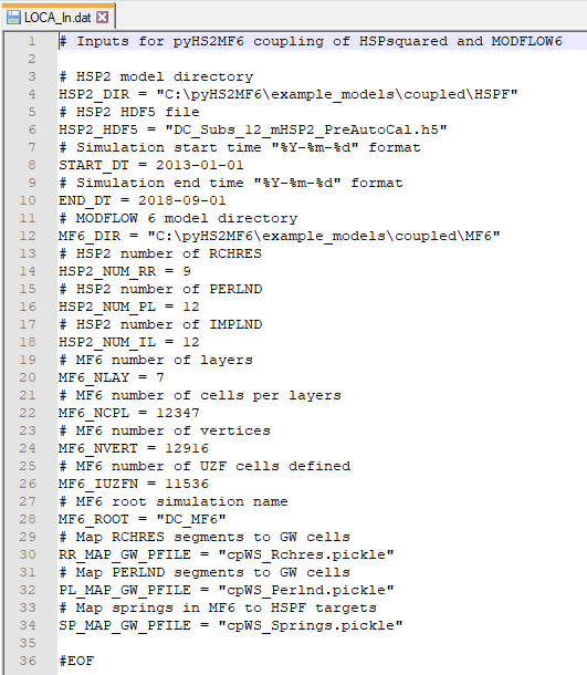
Example pyHS2MF6 input file

3.4.1.4. Spatial Mapping for Coupling

The primary purpose of this input file is to tell pyHS2MF6 where to find the spatial mapping information that allows mHSP2 to process the arrays that are passed back and forth between HSPF and MODFLOW 6. The indexes of these arrays are identified with MODFLOW 6 computational grid locations, and the mapping component tells mHSP2 how to transform the grid locations to HRUs and stream segments.

Three different mapping files need to be provided to pyHS2MF6.

1. RR_MAP_GW_PFILE pyHS2MF6_Inputs.RR_MAP_GW_PFILE: provides specification of groundwater model cells that correspond to each defined RCHRES in the model.

   • RCHRES exit number that goes to groundwater

   • Example cpWS_Rchres.pickle

2. PL_MAP_GW_PFILE pyHS2MF6_Inputs.PL_MAP_GW_PFILE: provides specification of groundwater model cells that correspond to the pervious parts of each HRU defined in the model.

   • Example cpWS_Perlnd.pickle

3. SP_MAP_GW_PFILE pyHS2MF6_Inputs.SP_MAP_GW_PFILE: defines the DRN cells that represents springs discharging to the ground surface within the HSPF model domain.

   • Example cpWS_Springs.pickle

Two examples of the creation of these three files are provided.

1. Jupyter Notebook pyHS2MF6_Create_Spatial_Mapping.

2. Jupyter Notebook Create_Coupled_Model_Mapping: the format for SP_MAP_GW_PFILE in this notebook is now out of date.

These Jupyter Notebooks also provide definition of the Python objects that compose these input files. The mapping files are saved as pickle files which provide a serialized version of of Python objects or variables. The top level objects in these input, mapping pickle files are dictionaries. One of the values in each dictionary entry is a pandas DataFrame. The DataFrame provides for the mapping between groundwater model cells and HSPF lumped parameter regions.

Included in the mapping are specification of weights for each cell. The purpose of these weights is to provide the ability to focus infiltration from an HRU or stream segment to a discrete feature or subset of cells in the groundwater model. Figure Spatial mapping weights provides a depiction of the spatial mapping weights used in the coupled model. The weights were specified to focus infiltration and seepage into the hydrologic soil type A, stream bed locations.

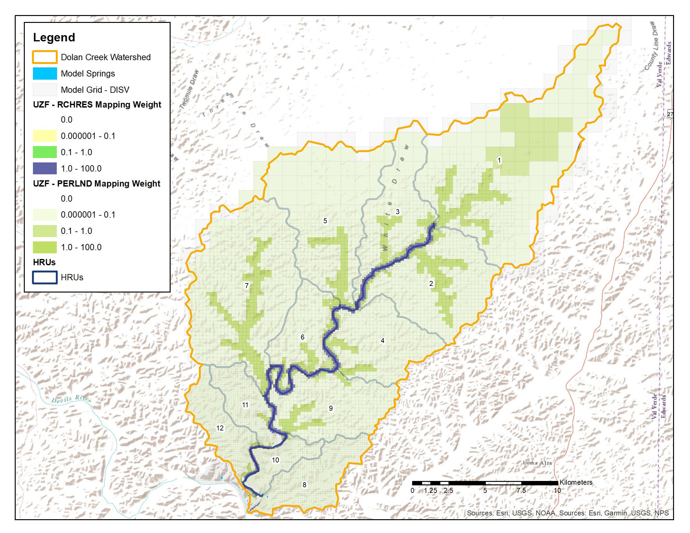
Spatial mapping weights

3.4.2. Coupled Mode Calibration and Results

In an actual scientific model application, the coupled model would be calibrated to water level measurements in wells and discharge observed at stream gauges. For this test case, a very basic manual, trial–and–error process was used to adjust the parametrization of the coupled model. The goal of these adjustments was to improve the match between the daily time series of Dolan Creek discharge (see Figure Standalone HSPF Model Results) from the gage record and simulated discharge from Reach #5. Standalone HSPF model parameters were not modified as part of these adjustments. In MODFLOW 6, hydraulic conductivity values, storage values, and DRN conductance were adjusted to improve the fit between pyHS2MF6 model results and the gage record.

Note

As stated earlier, an actual scientific model application to the study site would likely involve calibration to observed water level elevations in wells. This was not done for this case study because of time limitations, but pyHS2MF6 will support joint calibration to stream gage records and observed well water level elevations.

Figure Adjusted coupled model match to Dolan Creek discharge displays the simulated Reach #5 discharge for the adjusted, coupled model. The coupled model results provide a better match to the recession curves after each event relative to the standalone HSPF model.

Adjusted coupled model match to Dolan Creek discharge

3.4.2.1. Coupled Mode Results

pyHS2MF6 produces all of the outputs which are produced by MODFLOW 6 and HSPsquared. In addition, custom outputs are written to the mHSP2 HDF5 file and to four custom, pyMF6 pickle files.

The Jupyter Notebook pyHS2MF6_Coupled_Results_Example provides an example of processing these custom outputs. Additionally, this notebook provides definition of the the custom output structures. This notebook can be used as a template or building block for processing of the custom, coupled model outputs.

The primary purpose of these custom, coupled model outputs is to provide both a summary of the water exchanged between HSPF and MODFLOW 6 and a volume balance check to ensure that no water (or mass) is lost during the coupled simulation.

Note

Because pyHS2MF6 uses existing HSPF and MODFLOW 6 boundary condition logic and functionality, all custom outputs can be obtained from the individual HSPF and MODFLOW 6 outputs. However, the custom summarization is provided to facilite validation of simulation mass balance and to simplify identification of the exchanged water volumes and locations for exchange.

Deep percolation provides the primary link from HSPF to MODFLOW 6. Figure Simulated discharge from HSPF to MODFLOW 6 displays the average, deep percolation discharge sent from HSPF to MODFLOW 6. The focus of coupled model, water exchange is the dry stream beds which are mapped as hydrologic soil type A (see Figure Dolan Creek watershed).

Simulated discharge from HSPF to MODFLOW 6

An important check on coupled mode simulation results is to ensure that the water sent from HSPF is received by MODFLOW 6 and to confirm that surface discharge from MODFLOW 6 is received by HSPF. Figure Mass balance verification of infiltration sent from HSPF to MODFLOW 6 validates that all water sent from HSPF is received by MODFLOW 6. While, Figure Mass balance verification of surface discharge sent from MODFLOW 6 to HSPF confirms that discharge to the ground surface sent from MODFLOW 6 is received by HSPF.

Mass balance verification of infiltration sent from HSPF to MODFLOW 6

Mass balance verification of surface discharge sent from MODFLOW 6 to HSPF

3.4.3. Running a Coupled pyHS2MF6 Simulation

A coupled pyHS2MF6 simulation is executed from an Anaconda Prompt using the instructions below. For these instructions it is assumed, that pyHS2MF6 is installed at C:\pyHS2MF6, that the mHSP2 model input files are in the directory C:\Models\cp_mHSP2, that the pyMF6 model input files are in the directory C:\Models\cp_pyMF6, and that the coupled model input file, LOCA_In.dat, is in the directory C:\Models.

1. Activate the pyhs2mf6 Anaconda virtual environment. Additional details can be found at Anaconda Install Instructions.

   (base) > conda activate pyhs2mf6
   

2. Make the current directory the model directory.

   (pyhs2mf6) > cd C:\Models
   

3. Run the model

   (pyhs2mf6) > python C:\pyHS2MF6\bin\coupledMain.py LOCA_In.dat
   

The coupled model will create four log files that record general information and any issues encountered during the run.

1. C:\Models\sa_mHSP2\mHSP2_Log.txt: the mHSP2 log file

   • mHSP2_Log.txt

2. C:\Models\sa_MF6\pyMF6_Log.txt: the pyMF6 log file

   • pyMF6_Log.txt

3. C:\Models\pyHS2MF6_Log.txt: the coupled controller and queue server log file

   • pyHS2MF6_Log.txt

4. C:\ModelsMF6_ShellOut.txt: an echo of the MODFLOW 6 shell output that shows the current simulation time step

   • MF6_ShellOut.txt

The traditional MODFLOW 6 log files, .lst files, are still output by pyHS2MF6 and these provide MODFLOW-related troubleshooting information.