3.3. Standalone MODFLOW 6 Model

This case study application was developed to assist in pyHS2MF6 development and testing. There was not an existing MODFLOW 6 model to use as a starting point. A transient, standalone MODFLOW 6 model was created expressly for development and testing of pyHS2MF6.

A transient groundwater flow model is required because there is not a static version of an HSPF model. Consequently, a transient groundwater flow model is required for coupled mode simulation and so the standalone mode model should also be transient.

pyMF6 is the name of the standalone MODFLOW 6 component of pyHS2MF6. The pyMF6 code base is documented in pyMF6. pyMF6 has all of the functionality and uses all of the code base of MODFLOW 6.

The pyMF6 input files for the case study are on the GitHub site at standalone MODFLOW 6 input files These files are all standard MODFLOW 6 inputs and should work with any version of MODFLOW 6.

3.3.1. MODFLOW 6 Model Layout and Configuration

The study area is the Dolan Creek watershed which is composed of caprock mesas and dry arroyos. Dolan Creek is ephemeral until the lower-most stream segment, which is just above the confluence with the Devils River. The MODFLOW 6 model was created with seven computational layers covering the areal extent shown on Figure MODFLOW 6 layers and hydrostratigraphy. A DISV-style, unstructured grid is used for each layer. The computational grid was created using the USGS GridGen program.

Caution

The DISV-style grid is the only MODFLOW 6 grid option supported for coupled mode simulation. All MODFLOW 6 grid configurations are supported for standalone mode simulation.

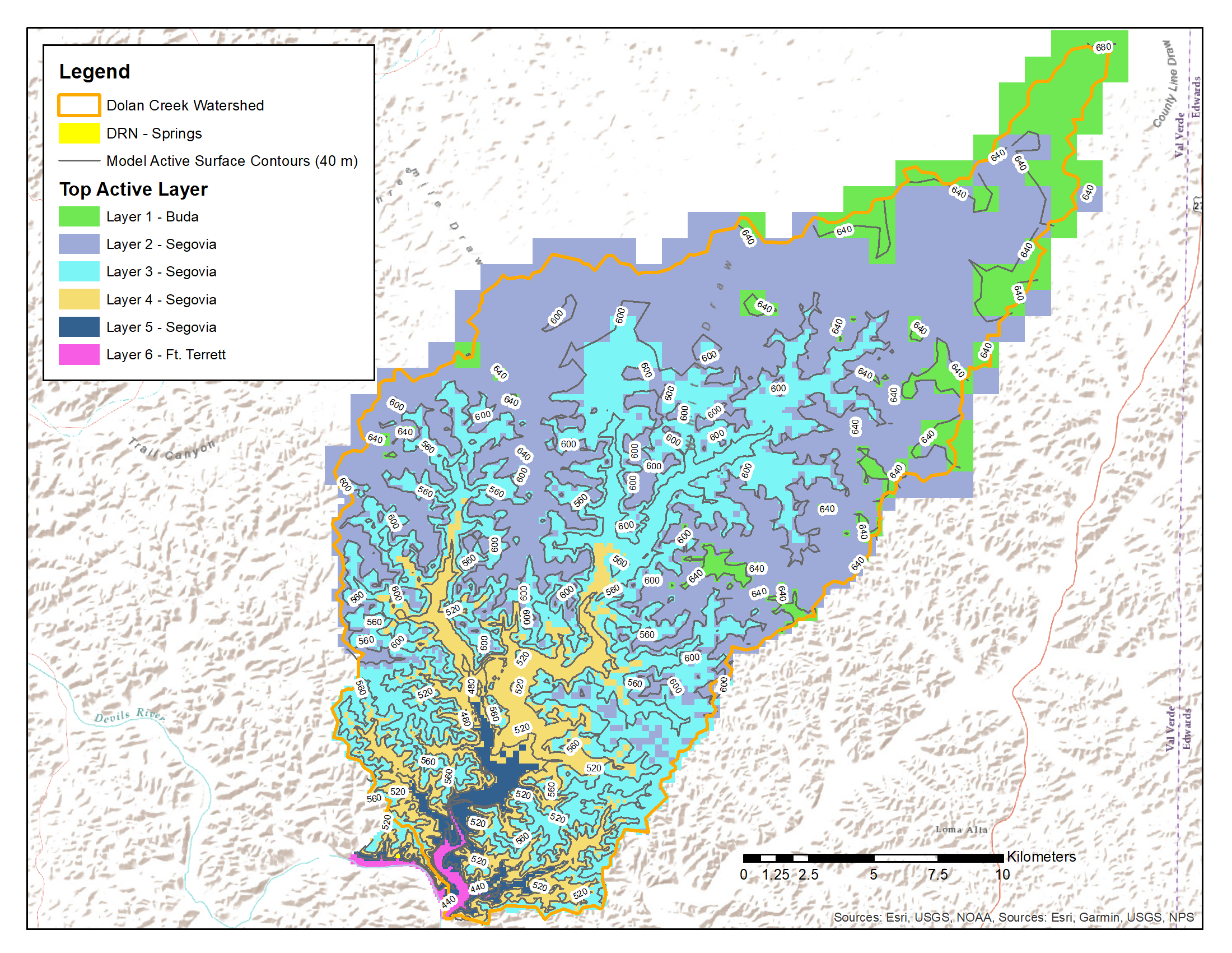
MODFLOW 6 layers and hydrostratigraphy

The seven computational layers are used to represent four different HSUs of the Edwards Formation. Each layer is flat and cells are inactivated to form depressions for stream valleys and dry arroyos. This effect can be seen in the color patterns denoting the valley bottoms in Figure MODFLOW 6 layers and hydrostratigraphy. Table MODFLOW 6 layers and HSUs provides the HSU and computational layer characteristics for each layer.

MODFLOW 6 layers and HSUs

Layer	HSU	Elevation Range (m)	Typical K (m/d)
1	Buda	685 - 635	0.1
2	Segovia	635 - 570	0.1
3	Segovia	570 - 510	1.0
4	Segovia	510 - 450	0.1
5	Segovia	450 - 420	1.0
6	Fort Terrett	420 - 390	0.05
7	Devils River	390 - 250	0.8

3.3.1.1. Boundary Conditions

Specific boundary condition types are required in the MODFLOW 6 model for coupling to HSPF. The requirements are enumerated below.

1. UZF Advanced Stress Package - required for all water transfers between programs where MODFLOW receives water from HSPF. The two primary cases where MODFLOW receives water are deep infiltration from the bottom of the soil column and stream leakage from the bottom of the stream bed.

2. DRN Stress Package - required to represent discharge of water to the ground surface from springs.

The UZF and DRN boundary conditions should also be used in the standalone model to represent pervious HRU areas, UZF, and springs, DRN.

Figure Standalone model boundary conditions shows locations for all boundary condition, or stress package, types used in the standalone model. The boundary condition types, not yet discussed, are listed below.

• RIV Stress Package - represents stream segments that are represented in the HSPF model with RCHRES structures.

• RCH Stress Package - represents pervious land segments that are outside of the HSPF model domain.

• GHB Stress Package - provides or enforces a regional flow pattern at the groundwater model domain edges.

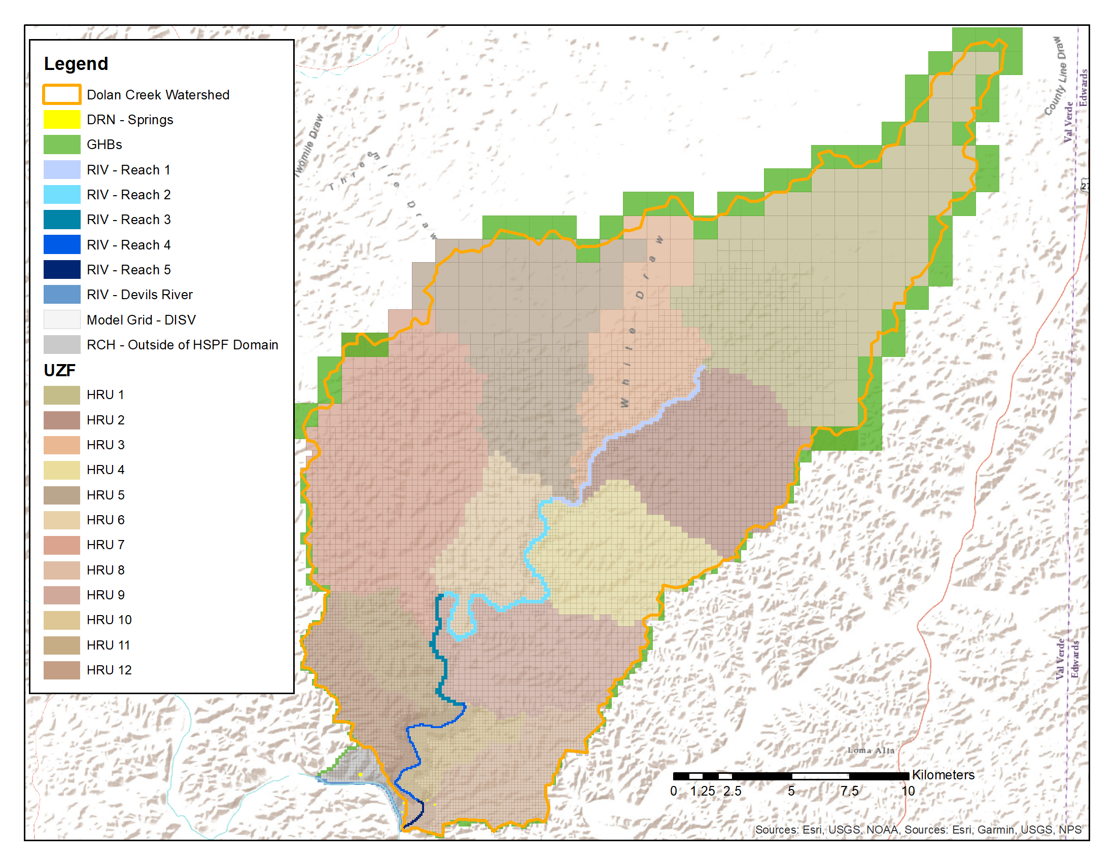
Standalone model boundary conditions

In Figure Standalone model boundary conditions the UZF and RIV boundary conditions are labeled according to corresponding HSPF structures. The MODFLOW 6 OBS package is used to collate and track water budget information for these identified regions for comparison to the standalone HSPF model results as part of calibration.

As the standalone MODFLOW 6 model needs to be transient and water will be passed back and forth between HSPF and MODFLOW each simulation day in coupled mode, time-series records are used to specify stress package forcing for RIV, RCH, and UZF. The time-series forcing is correlated to precipitation so that RCH and UZF only represent infiltration associated with rainfall and so that RIV only represents water in Reaches #1 - #4 associated with rainfall.

It is important to provide this daily, time-series forcing in semi-arid environments in order to facilitate configuration of the Newton-Raphson solver formulation and the UZF wave sets. The Newton-Raphson solver will provide a better representation of the dynamic water table movements expected for the semi-arid, karst terrain study site.

3.3.2. Standalone Calibration

Ideally, an existing, standalone MODFLOW 6 model would be calibrated as part of a previous study. As this is a test model to provide a coupling example, a calibration was not completed for this test model. A trial–and–error approach was employed to approximately match the external inflow time series for Reach #5 in the standalone HSPF model with simulated spring discharge from Dolan Springs and YR-70-01-701 (see Figure Dolan Creek watershed).

Note

All of the standard MODFLOW 6 capabilities are available in pyMF6. For a real modeling study, the MODFLOW 6 model would also be calibrated to observed water levels in wells. This would be done with whatever means is preferred by the modeler and could include PEST or other automated, parameter estimation tool.

Figure Standalone model calibration displays the match between simulated spring discharge in the MODFLOW 6 model and the external time series used to introduce spring discharge to Reach #5 in the HSPF model.

Standalone model calibration

To achieve, this level of spring discharge in the MODFLOW 6 model, a preferential flow pathway was added to the eastern side of the domain which funnels water to these springs. The location of this preferential pathway is shown on Figure Preferential flow pathway.

Caution

The need for the preferential pathway is somewhat determined by the domain geometry for this case study model. In this model, the groundwater flow model domain is largely coincident with the Dolan Creek watershed. Setting a groundwater flow model domain to be coincident with the surface water watershed for the stream of interest is never a good idea; the domain boundaries should always be extended away from the focus area to avoid boundary effects.

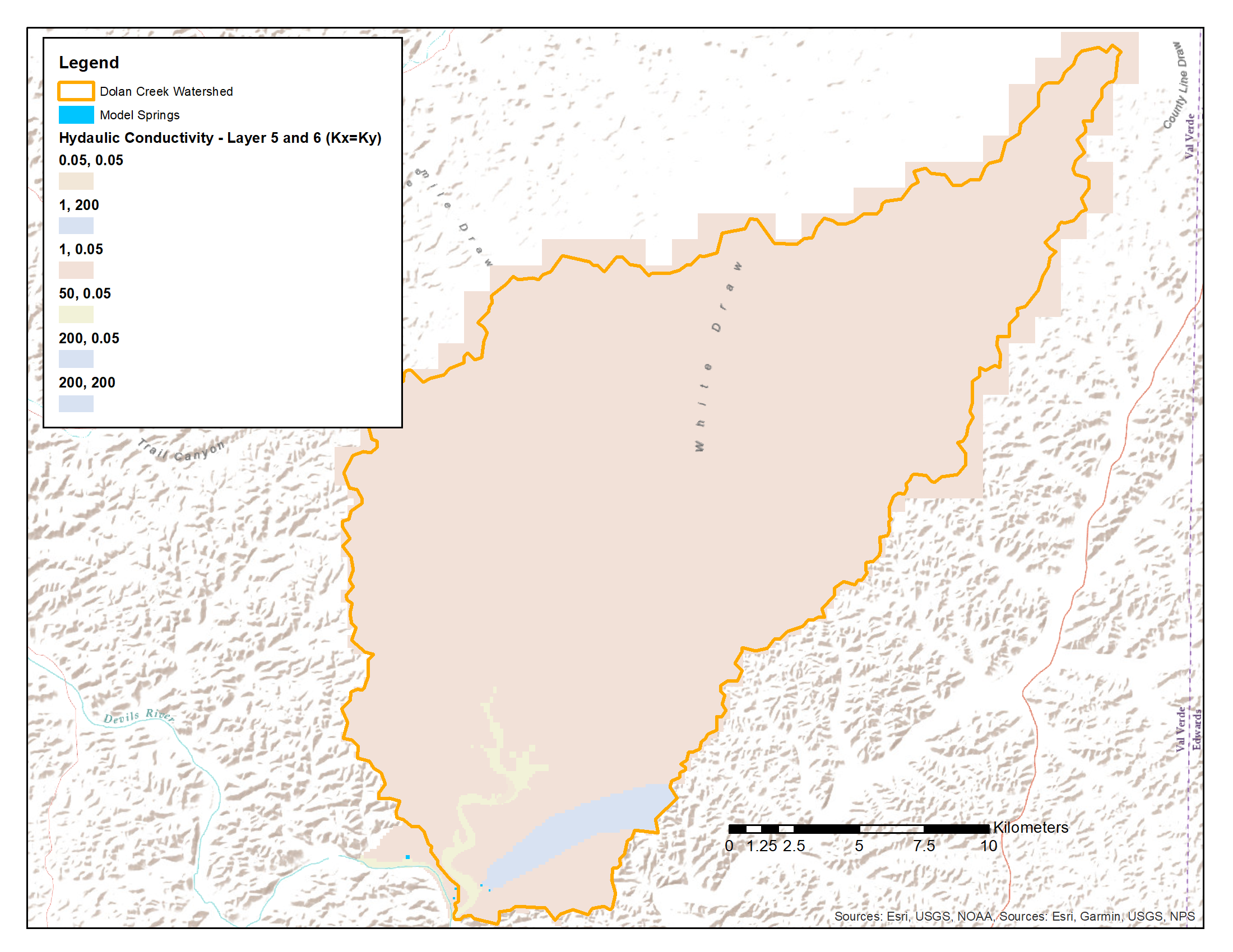
Preferential flow pathway

The simulated water levels at the end of the transient, standalone, groundwater flow model simulation are shown on Figure Simulated groundwater levels along with the depth to the water table. Simulated water levels are close to the ground surface in the stream valleys, especially as move downstream to the Reach #4 and #5 regions. Bounding the groundwater flow domain with the surface water watershed contributes to this effect. The shape of the domain is arbitrarily focusing groundwater flow to Reach #4 and #5.

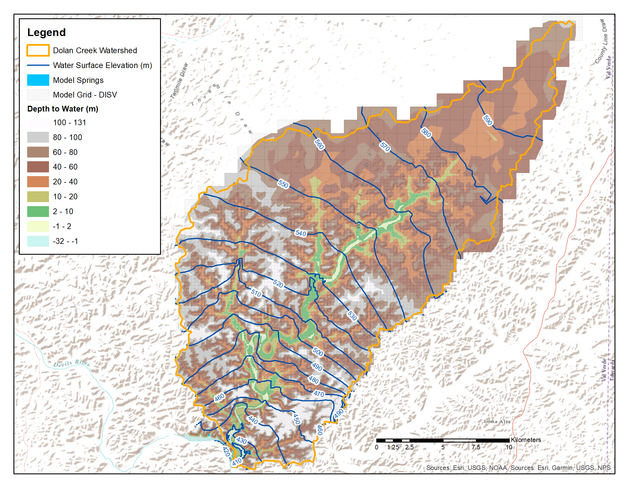
Simulated groundwater levels

3.3.3. Running a Standalone pyMF6 Simulation

A standalone pyMF6 simulation is executed from an Anaconda Prompt using the instructions below. For these instructions it is assumed, that pyHS2MF6 is installed at C:\pyHS2MF6 and that the model input files are in the directory C:\Models\sa_MF6.

1. Activate the pyhs2mf6 Anaconda virtual environment. Additional details can be found at Anaconda Install Instructions.

   (base) > conda activate pyhs2mf6
   

2. Make the current directory the model directory.

   (pyhs2mf6) > cd C:\Models\sa_MF6
   

3. Run the model

   (pyhs2mf6) > python C:\pyHS2MF6\bin\standaloneMain.py MF6 C:\\Models\\sa_MF6 -f mfsim.nam
   

The model will create a log file that records general information and any issues encountered during the run. The standalone pyMF6 log file generally contains little information. The traditional MODFLOW 6 log files, .lst files, are output by pyMF6 and these provide any troubleshooting information that may be required.

For the example provided above, the run log is written to the file C:\Models\sa_MF6\pyMF6_Log.txt. An example pyMF6_Log.txt is available in the standalone, example model directory.

In terms of accessing standalone simulation results, pyMF6 produces the same outputs as generated by MODFLOW 6. The modeler should use their normal tools for post-processing MODFLOW 6 output.