3.2. Standalone HSPF Model
This case study application was developed to assist in pyHS2MF6 development and testing. The only existing HSPF model that was available to use as a starting point was created for a separate study examining water resources risk from climate change (Martin 2020). This standalone HSPF model was used as the starting point for testing pyHS2MF6.
mHSP2 is the name of the standalone HSPF component of pyHS2MF6. The mHSP2 code base is documented in mHSP2. It uses the same input file format as used by the HSPsquared variant of HSPF.
The mHSP2 input file for the case study is a HDF5 file. This standalone mHSP2 input file is available on the pyHS2MF6 GitHub site.
3.2.1. HSPF Model Layout and Configuration
The site watershed was divided into 12 sub-watershed,
HRUs. Each HRU has PERLND, pervious
land, and IMPLND, impervious land, components or areas. IMPLND areas are
composed of gravel roads and structures. Given the limited development
in this area, the pervious land area is >> impervious land area.
Five RCHRES, stream reach or well mixed reservoirs, are used to route water from the upstream-most HRU to the watershed outlet. RCHRES #5 is the stream segment where the stream gage and the springs are located. This reach is hypothesized to be a gaining stream reach where external water enters the reach from springs in addition to the water that is routed downstream from Reach #4. Reaches #1 - #4 are hypothesized to be losing reaches.
An important conceptualization for coupled model simulation is how to treat gaining and losing reaches for communication with the groundwater flow model. Gaining and losing requires different HSPF configurations to facilitate future coupling to a groundwater flow model.
Gaining reaches: additional input water from spring discharge or other baseflow components is input to a RCHRES structure as an external inflow time series.
This is the treatment used for Reach #5 to represent contributions from Dolan Springs and YR-70-01-701.
Losing reaches: In HSPF, there is not a preconfigured process for stream losses to groundwater because saturated groundwater conditions are not really represented in HSPF. The representation of loses from stream segments to groundwater is then largely up to the modeler. In pyHS2MF6 the modeler should specify one RCHRES exit to represent loses to groundwater. Typically, one RCHRES exit is used to calculate downstream discharge that is routed to the next RCHRES downstream and one RCHES exit is used to remove water from the model that represents loses to groundwater.
In the standalone HSPF model, exit #2 for Reaches #1 - #4 represents seepage to groundwater from the stream. HSPF calculates this seepage using a volume-based, or FTAB, calculation for the standalone model. This volume-based, seepage relationship was manually adjusted to improve the match between simulated discharge at the watershed outlet and gage discharge.
If desired, the user can implement a time-based relationship for discharge from an exit. Consequently, a time-based relationship could be used for exit #2 to represent seepage to groundwater.
Note
A single reach can be represented as both gaining and losing using both a specified external time series inflow and an outflow calculation for a designated exit for discharge to groundwater. This is not recommended. The recommended approach would be to use two RCHRES for the stream segment with one portraying gaining conditions and one representing losing conditions.
Figure HSPF model configuration shows the HSPF model layout for the study site. Complete details of HSPF model configuration are available in the standalone mHSP2 input file.
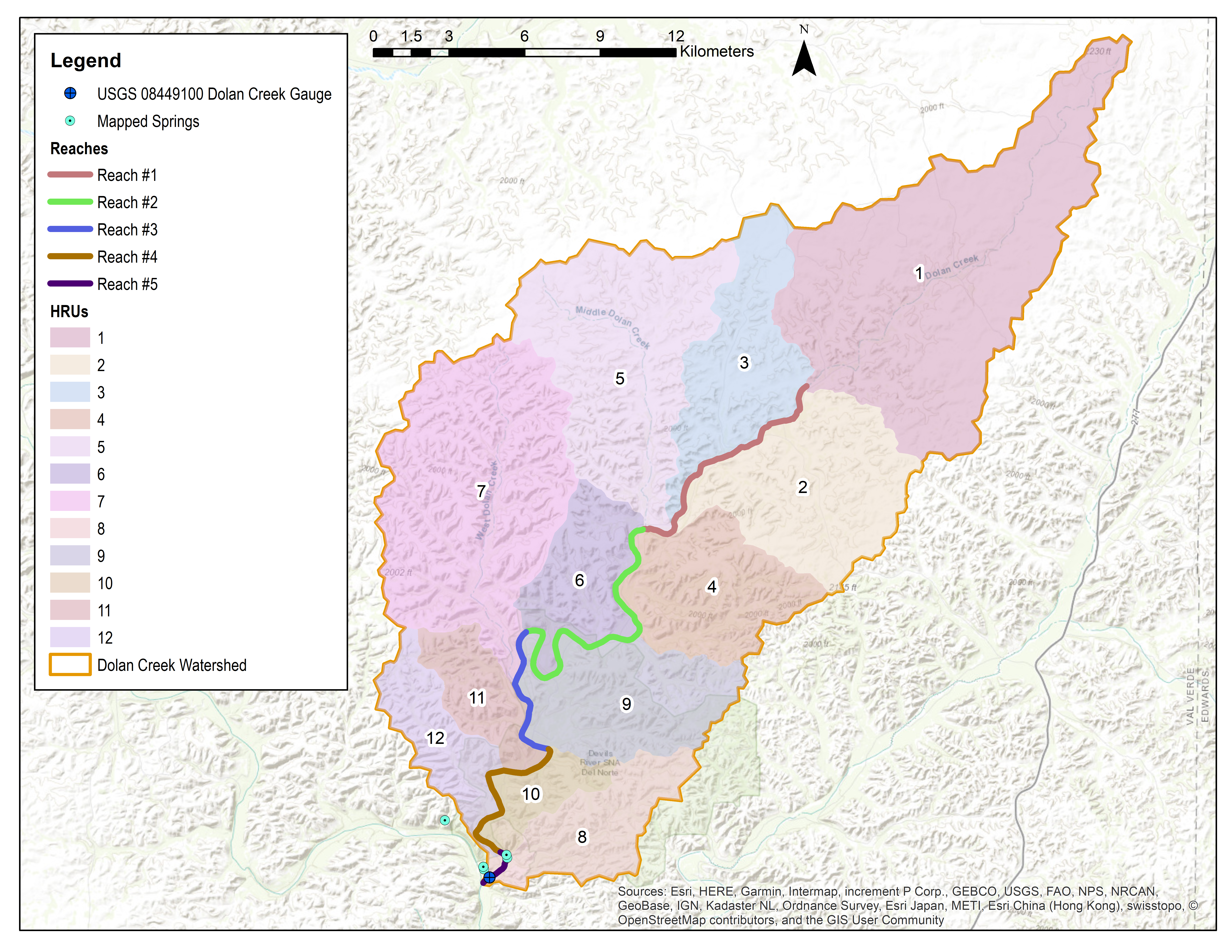
HSPF model configuration
Adapted from “Watershed-Scale, Probabilistic Risk Assessment of Water Resources Impacts from Climate Change” by N. Martin, 2021. water, v. 13. CC BY 4.0
3.2.1.1. Calibration
The goal for the standalone model is to produce Reach #5 outflow that approximately represents the observed Dolan Creek stream flow discharge from USGS Gage 08449100. Ideally, an existing, standalone HSPF model would be calibrated as part of a previous study. For test model formulation, the standalone HSPF model was employed directly as available from Martin (2020).
In this model, estimates of spring discharge from Dolan Springs and YR-70-01-701 (see Figure Dolan Creek watershed) are provided to the HSPF model as an external time series of inflows to Reach #5. Simulation results for the standalone HSPF model are shown on Figure Standalone HSPF Model Results. In this figure, the orange shaded area denotes the estimated, external inflow time series to Reach #5 that represents the combination of Dolan Springs and YR-70-01-701 discharge.

Standalone HSPF Model Results
Adapted from “Watershed-Scale, Probabilistic Risk Assessment of Water Resources Impacts from Climate Change” by N. Martin, 2021. water, v. 13. CC BY 4.0
3.2.2. HSPF Software Packages and Conversion
The standalone HSPF model was created using the following combinations of HSPF-variant software.
The initial HSPF model set-up and configuration were implemented using PyHSPF. This produces a HSPF UCI file and input and output WDM files.
HSPsquared was then employed to convert the UCI file and input WDM file to an HSPsquared input HDF5 file. This format is similar to what is required for mHSP2.
Next, the Jupyter Notebook mHSP2_SetSaves was employed to modify the HSPsquared, input HDF5 file to be provide the specification of model outputs that is required by mHSP2.
3.2.3. Running a Standalone mHSP2 Simulation
A standalone mHSP2 simulation is executed from an Anaconda Prompt using the instructions below. For these instructions it is assumed, that pyHS2MF6 is installed at C:\pyHS2MF6 and that the model HDF5 file is in the directory C:\Models\sa_mHSP2.
Activate the pyhs2mf6 Anaconda virtual environment. Additional details can be found at Anaconda Install Instructions.
(base) > conda activate pyhs2mf6
Make the current directory the model directory.
(pyhs2mf6) > cd C:\Models\sa_mHSP2
Run the model
(pyhs2mf6) > python C:\pyHS2MF6\bin\standaloneMain.py HSP2 C:\\Models\\sa_mHSP2 -f DC_CalibmHSP2.h5
The model will create a log file that records general information and any issues encountered during the run. The log file provides a listing of input parameters along with required units. It also provides a listing of output parameters along with output units.
For the example provided above, the run log is written to the file C:\Models\sa_mHSP2\mHSP2_Log.txt. An example mHSP2_Log.txt is available in the standalone, example model directory.
In terms of accessing standalone simulation results, the Jupyter Notebook mHSP2_SA_Results provides a simple example of extracting and analyzing standalone mHSP2 results.